My First R Package: halfplus7

Development

Projects

Packages

I developed my first R package!

Author

Sydney Lewis

Published

January 1, 2024

Introduction

In my Statistical Programming Paradigms and Workflows course, one of our projects was to create a pkgdown site for an R package. If we wanted, we had the opportunity to use a package that we had created for this project, instead of a package developed by another person. Going into this class, I wouldn’t have expected that I would create an original R package and I feel proud that I took the plunge to develop one.

I was inspired by a Tidy Tuesday data set with Age Gaps for Hollywood Movie Couples. This gave me the idea to create a package that included some basic mathematical formulas to apply to “Half-Your-Age-Plus-7” Rule (also called the “Standard Creepiness Rule”), which is used to determine the appropriateness (or creepiness) of an age difference in a couple. As the Rule suggests, in order to determine the lowest age that someone may date, they would take half of their age and add 7. For example, a person who is 30 years old would then be able to date someone as young as 22 (30 / 2 + 7 = 22). This was a silly concept, but it was a great start to help me practice my development skills and create a new R package.

You can learn more about my halfplus7 package at my pkgdown site.

Functions

Below are a list of the currently available functions in the halfplus7 package. There are additional vignettes for these functions on the pkgdown site.

lower_limit : This function provides the lower age limit for a given age, returning a numeric value.

Code

library(halfplus7)

lower_limit(50)

[1] 32

upper_limit : This function provides the upper age limit for a given age, also returning a numeric value.

Code

upper_limit(35)

[1] 56

age_range : This function provides the appropriate age range for a given age, returning two numeric values (lower_limit and upper_limit).

Code

age_range(42)

lower_limit upper_limit 
         28          70

check_couple : This function provides a verdict about a couple, given their two ages. This will return TRUE if the paired ages meet the Rule and FALSE when they do not.

Code

check_couple(20, 70)

[1] FALSE

Code

check_couple(30, 27)

[1] TRUE

ages_firstok : This function provides the ages when a couple would first meet the Rule, given their birth dates. This returns two numeric values representing the youngest ages for the two people.

Code

ages_firstok("1722-02-22", "1858-10-27")

  Age of Older Person Age of Younger Person 
             287.3470              150.6735

Again, the full details on the halfplus7 package are available at the pkgdown site. Below, I have included additional examples for how to use the package’s functions with a dataset that includes many Hollywood movie couples.

Examples with Hollywood Movie Couples

The code below includes loading the tidyverse and halfplus7 packages, downloading the data from GitHub, and cleaning the data for the later visualizations. The data used are from a Tidy Tuesday data set with Age Gaps for Hollywood Movie Couples.

Code

library(tidyverse)

download_and_save <- function(file_name, url) {
  data_folder <- "data"
  file_path <- file.path("data", file_name)
  # See if the file already exists
  if (!file.exists("data")) {
    dir.create("data", recursive = TRUE)
  }
  if (!file.exists(file_path)) {
    # Download the data if it does not exist
    data <- readr::read_csv(url)
    # Saves the data to the path with the desired name
    write.csv(data, file = file_path, row.names = FALSE)
  }
}

# Uses download_and_save function with age_gaps.csv from GitHub
download_and_save("age_gaps.csv", 'https://raw.githubusercontent.com/rfordatascience/tidytuesday/master/data/2023/2023-02-14/age_gaps.csv')

# Imports raw age_gap dataset
age_gaps_raw <- read_csv("data/age_gaps.csv")

age_gaps_v1 <- age_gaps_raw %>%
  # creates new variable to describe sexual orientation of couple
  mutate(orientation = ifelse(character_1_gender == "man" & character_2_gender == "man" |
                               character_1_gender == "woman" & character_2_gender == "woman",
                             "LGBTQ",
                             "Straight"),
         # modifies birthdate variables to be treated as dates
         actor_1_birthdate = ymd(actor_1_birthdate),
         actor_2_birthdate = ymd(actor_2_birthdate))

#calculates the older actor in the couple
calculate_older_actor <- function(man_birthdate, woman_birthdate) {
  if (man_birthdate < woman_birthdate) {
    return("man")
  } else if (woman_birthdate < man_birthdate) {
    return("woman")
  } else {
    return("same birthdate")
  }
}

assign_gender_details <- function(character_1_gender, character_2_gender, actor_1_age, actor_1_birthdate, actor_1_name, actor_2_age, actor_2_birthdate, actor_2_name) {
  details <- list()

  if (character_1_gender == "man") {
    details$man_age <- actor_1_age
    details$man_birthdate <- ymd(actor_1_birthdate)
    details$man_name <- actor_1_name
  } else {
    details$man_age <- actor_2_age
    details$man_birthdate <- ymd(actor_2_birthdate)
    details$man_name <- actor_2_name
  }

  if (character_2_gender == "woman") {
    details$woman_age <- actor_2_age
    details$woman_birthdate <- actor_2_birthdate
    details$woman_name <- actor_2_name
  } else {
    details$woman_age <- actor_1_age
    details$woman_birthdate <- actor_1_birthdate
    details$woman_name <- actor_1_name
  }

  return(details)
}

age_gaps_straight <- age_gaps_v1 %>%
  filter(orientation == "Straight") %>%
  mutate(
    details = pmap(list(character_1_gender, character_2_gender, actor_1_age, actor_1_birthdate, actor_1_name, actor_2_age, actor_2_birthdate, actor_2_name), assign_gender_details)
  ) %>%
  # Unpack the details
  mutate(
    man_age = map_dbl(details, "man_age"),
    man_birthdate = map(details, "man_birthdate") %>% map_chr(as.character) %>% ymd(),
    man_name = map_chr(details, "man_name"),
    woman_age = map_dbl(details, "woman_age"),
    woman_birthdate = map(details, "woman_birthdate") %>% map_chr(as.character) %>% ymd(),
    woman_name = map_chr(details, "woman_name"),
    older_actor = pmap_chr(list(man_birthdate, woman_birthdate), calculate_older_actor)
  ) %>%
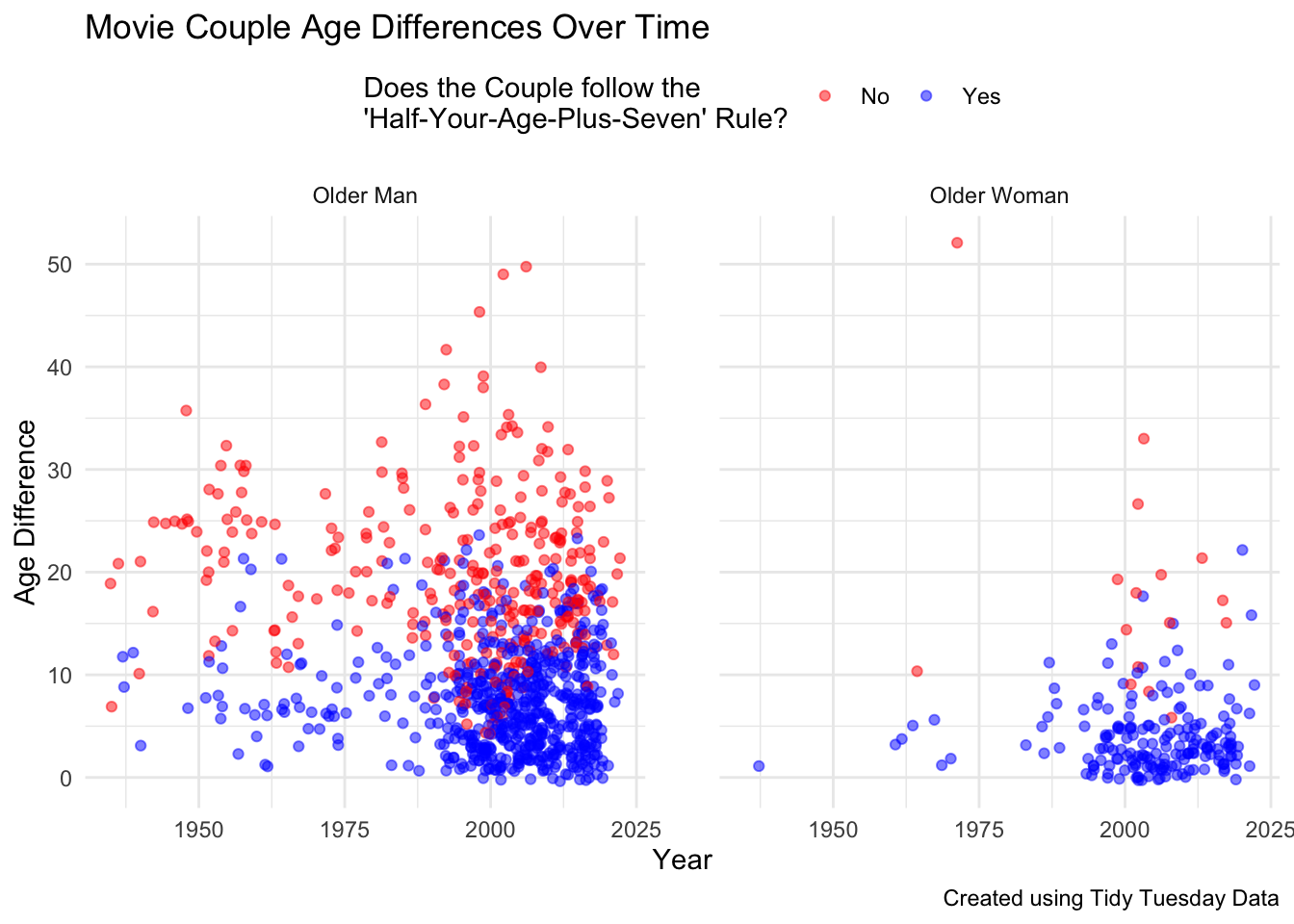
  select(-details)

Age Differences over Time in Hollywood Movie Couples

In this visualization, I only included straight couples and I faceted by the gender of the older actor in the couple. This visualization illustrates how there are fewer movie couples where the older actor is a woman.

What is faceting?

Faceting is a great technique with data visualizations because it gives you another opportunity to stratify data by an additional variable. When you facet a plot by a variable, you would reproduce the plot with the groups separated by that variable. In the plot here, I facet by the gender of the older actor in the couple. Because there are only two options for gender in this data set, the output is two plots with one for when a man is the older actor in the couple and one when the woman is the older actor in the couple.

I used the check_couple function from my halfplus7 package to add information about whether these couples meet the “Half-Your-Age-Plus-7” Rule.

Code

age_gaps_straight %>%
  mutate(match_rule = case_when(
    check_couple(man_age, woman_age) == FALSE ~ "No",
    check_couple(man_age, woman_age) == TRUE ~ "Yes")) %>%
ggplot(aes(x = release_year, y = age_difference, color = match_rule)) +
  # adds jitter for discrete data
  geom_jitter(alpha = 0.5) +
  # designates color of points by gender of older actor in couple
  scale_color_manual(values = c("Yes" = "blue", "No" = "red")) +
  # creates labels for plot
  labs(
    title = "Movie Couple Age Differences Over Time",
    x = "Year",
    y = "Age Difference",
    color = "Does the Couple follow the \n'Half-Your-Age-Plus-Seven' Rule?",
    caption = "Created using Tidy Tuesday Data"
  ) +
  theme_minimal() +
  facet_wrap(~older_actor, labeller = labeller(older_actor = c("man" = "Older Man", "woman" = "Older Woman"))) + 
  theme(legend.position = "top",
        panel.spacing = unit(2, "lines"))

Has the size of age differences changed over time?

When to Use Simple Linear Regression

Simple Linear Regression makes sense to use when we have a continuous dependent variable and a continuous independent variable.

In this case, age difference is our dependent variable and release year is our independent variable. Both of these are continuous numeric variables. Because we are not including any other variables in our model, we would use a simple, rather than multiple, linear regression.

It appears that the average age difference has become smaller over time. I used a simple linear regression to determine whether there is a statistically significant difference in age differences across release years. Based on the results below (negative coefficient with p-value < 0.05), we would conclude that age differences have decreased over time and this trend is statistically significant.

Code

lin_model = lm(formula = age_difference  ~ release_year, data = age_gaps_v1)
summary(lin_model)


Call:
lm(formula = age_difference ~ release_year, data = age_gaps_v1)

Residuals:
    Min      1Q  Median      3Q     Max 
-16.203  -6.531  -2.022   4.844  40.128 

Coefficients:
              Estimate Std. Error t value Pr(>|t|)    
(Intercept)  223.00941   29.99798   7.434 2.05e-13 ***
release_year  -0.10625    0.01499  -7.087 2.38e-12 ***
---
Signif. codes:  0 '***' 0.001 '**' 0.01 '*' 0.05 '.' 0.1 ' ' 1

Residual standard error: 8.335 on 1153 degrees of freedom
Multiple R-squared:  0.04174,   Adjusted R-squared:  0.04091 
F-statistic: 50.22 on 1 and 1153 DF,  p-value: 2.384e-12

Has the proportion of movie couples who meet the Rule increased over time?

Looking at the above visualization, I also hypothesize that the proportion of movie couples who meet the Rule has increased over time; however, the amount of movies also appears to have increased. I am curious if there is a statistically significant trend in the proportion of couples meeting the “Half-Your-Age-Plus-7” Rules over time. In answering this question, I will use simple logistic regression.

When to Use Simple Logistic Regression

Simple Logistic Regression makes sense to use when we have a binary dependent variable and a continuous independent variable.

In this case, whether the couple meets the “Half-Your-Age-Plus-7” Rule is our dependent variable and release year is our independent variable. Our dependent variable is binary and our independent variable is continuous. Because we are not including any other variables in our model, we would use a simple, rather than multiple, logistic regression.

With the information below, it does appear the the proportion of Hollywood movie couples who meet the “Half-Your-Age-Plus-7” Rule has increased over time. The p-value is less than 0.05, which indicates that this trend is statistically significant.

Code

age_gaps_straight_log <- age_gaps_straight %>%
  # demonstrates check_couple function from halfplus7 package
  mutate(match_rule = case_when(
    # codes 0 when couple does not meet Rule
    check_couple(man_age, woman_age) == FALSE ~ 0,
    # codes 1 when couple does meet Rule
    check_couple(man_age, woman_age) == TRUE ~ 1))

rule_by_year_model = glm(formula = match_rule ~ release_year, data = age_gaps_straight_log, family = binomial(link = "logit"))
summary(rule_by_year_model)


Call:
glm(formula = match_rule ~ release_year, family = binomial(link = "logit"), 
    data = age_gaps_straight_log)

Coefficients:
               Estimate Std. Error z value Pr(>|z|)    
(Intercept)  -52.772643   7.789305  -6.775 1.24e-11 ***
release_year   0.026865   0.003897   6.893 5.46e-12 ***
---
Signif. codes:  0 '***' 0.001 '**' 0.01 '*' 0.05 '.' 0.1 ' ' 1

(Dispersion parameter for binomial family taken to be 1)

    Null deviance: 1344.4  on 1131  degrees of freedom
Residual deviance: 1295.7  on 1130  degrees of freedom
AIC: 1299.7

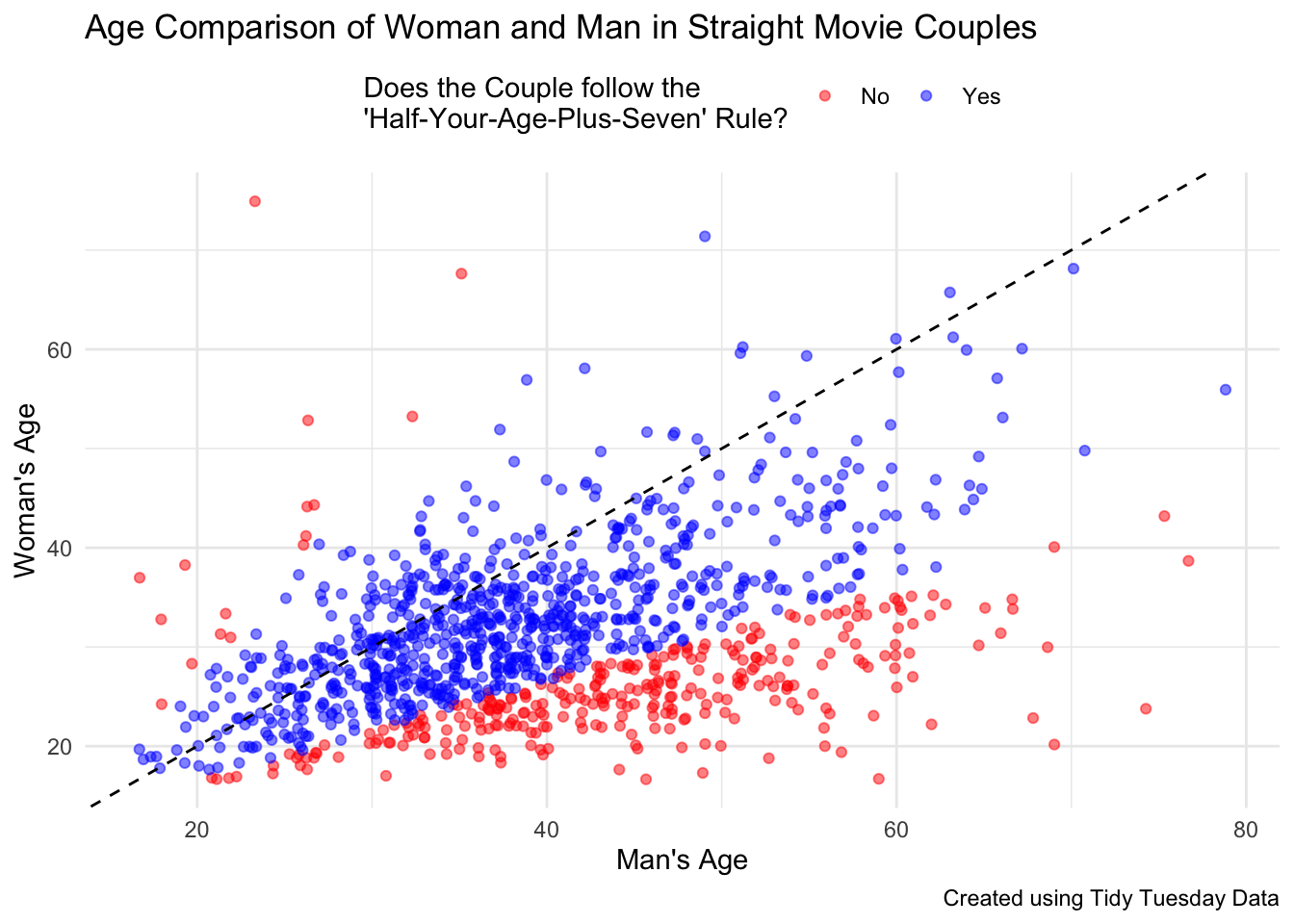
Number of Fisher Scoring iterations: 4

Age Comparison of Men and Women in Hollywood Movie Couples

This next visualization adds a different perspective for similar data.

Again, I used the check_couple function from my halfplus7 function to add information about whether these couples meet the “Half-Your-Age-Plus-7” Rule.

Code

age_gaps_straight %>%
  # demonstrates check_couple function from halfplus7 package
  mutate(match_rule = case_when(
    check_couple(man_age, woman_age) == FALSE ~ "No",
    check_couple(man_age, woman_age) == TRUE ~ "Yes")) %>%
  ggplot(aes(man_age, woman_age, color = match_rule)) +
  # adds jitter for discrete data
  geom_jitter(alpha = 0.5) +  
  # adds line at y = x to illustrate couples with the same age
  geom_abline(intercept = 0, slope = 1, linetype = "dashed", color = "black") +
  # designates colors to identify whether couple meets 'Half-Your-Age-Plus-7' Rule
  scale_color_manual(values = c("Yes" = "blue", "No" = "red")) +
  theme_minimal() +
  # adds labels for plot
  labs(
    title = "Age Comparison of Woman and Man in Straight Movie Couples",
    x = "Man's Age",
    y = "Woman's Age",
    color = "Does the Couple follow the \n'Half-Your-Age-Plus-Seven' Rule?",
    caption = "Created using Tidy Tuesday Data"
  ) + 
  # moves legend to top of plot
  theme(legend.position = "top")

Are couples where women are older than the man more likely to meet the Rule?

Based on the above visualization, I hypothesize that when you compare couples with an older man versus an older woman, the couple is more likely to meet the Rule when the woman is older. Of course, there are many more couples with older men, so this is difficult to determine from the visualized data. In answering this question of statistical significance, I will use a Chi-Square Test.

When to Use Chi-Square Test

Chi-Square Test is best to use when you have categorical variables and want to test the association between these two variables.

In this case, whether the couple meets the “Half-Your-Age-Plus-7” Rule and the sex of the older actor are both categorical variables.

Below is a 2x2 table with information about the gender of the older actor and whether the couple meets the Rule. In this table, the proportion of couples that do not meet the Rule is larger among couples with an older man than those with an older woman.

Code

age_gaps_straight_chi <- age_gaps_straight %>%
  # demonstrates check_couple function from halfplus7 package
  mutate(match_rule = case_when(
    # codes 0 when couple does not meet Rule
    check_couple(man_age, woman_age) == FALSE ~ 0,
    # codes 1 when couple does meet Rule
    check_couple(man_age, woman_age) == TRUE ~ 1))

xtabs(~ older_actor + match_rule, data = age_gaps_straight_chi)

           match_rule
older_actor   0   1
      man   302 627
      woman  16 187

Below are the results of the Chi-Square Test. As we observe, the p-value is very small (0.000000000001525). With this finding, we would reject the null hypothesis, which was that the proportion of couples meeting the rule was the same in couples with an older man and older woman, and conclude that these proportions are different. In other words, straight Hollywood movie couples with an older woman are more likely to meet the “Half-Your-Age-Plus-7” Rule than couples with an older man.

Code

chisq.test(xtabs(~ older_actor + match_rule, data = age_gaps_straight_chi), correct = FALSE)


    Pearson's Chi-squared test

data:  xtabs(~older_actor + match_rule, data = age_gaps_straight_chi)
X-squared = 50.016, df = 1, p-value = 1.525e-12

Couples with the 20 Largest Age Gaps

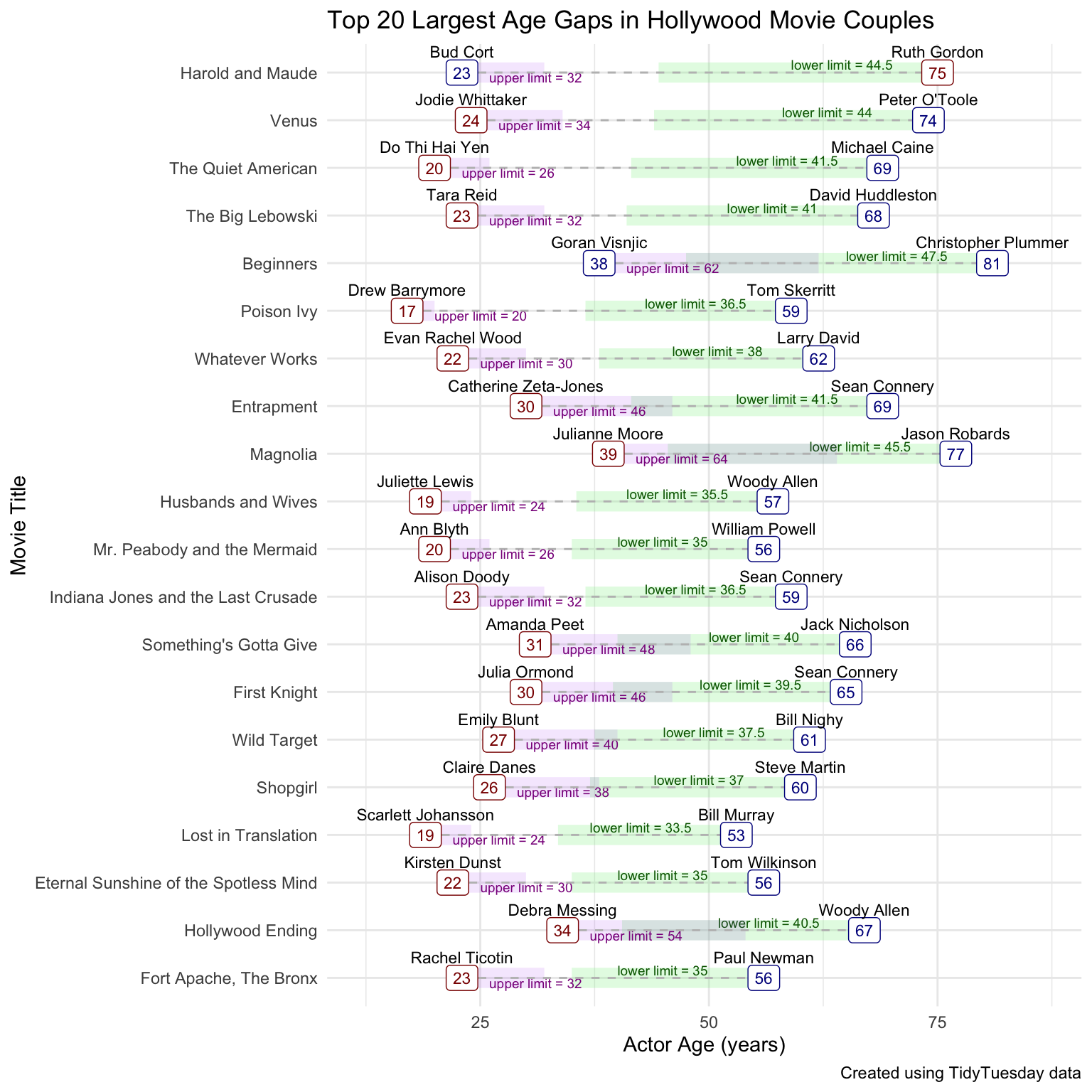
In the twenty largest age gaps when the man is older, none of women are within the lower age limit produced by the “Half-Your-Age-Plus-7” Rule.

The green shaded segments illustrate the lower age range for older actor, given the ‘Half-Your-Age-Plus-7’ Rule. The purple shaded segments illustrate the upper range for the younger actor. Because none of these couples meet the “Half-Your-Age-Plus-7” Rule, these shaded segments do not overlap with the other actor. In some of these cases, the shaded segments for the pair do not even overlap.

While the majority of these couples are straight couples with an older man and younger woman, the couple with the largest age difference has a older woman and a younger man. There is also a couple with two men included in this list.

I used the upper_limit and lower_limit functions from my halfplus7 package to create this visualization.

Code

top_age_gaps <- age_gaps_v1 %>%
  arrange(desc(age_difference)) %>%
  slice_head(n = 20) 

# modifies dataset above 
top_age_gaps_long <- top_age_gaps %>%
  uncount(weight = 1) %>%
  pivot_longer(cols = c(actor_1_age, actor_2_age), 
               names_to = "actor", 
               values_to = "age") %>%
  mutate(actor_name = ifelse(actor == "actor_1_age", actor_1_name, actor_2_name),
         actor_gender = ifelse(actor == "actor_1_age", character_1_gender, character_2_gender),
         age_lowerlim = lower_limit(age),
         age_upperlim = upper_limit(age))

top_age_gaps_long <- top_age_gaps_long %>%
  group_by(movie_name) %>%
  mutate(text_offset = seq(-0.3, 1, length.out = n())) %>%
  ungroup() %>%
  arrange(age_difference) %>%
  mutate(movie_name = factor(movie_name, levels = unique(movie_name)))

top_age_gaps_long %>%
  ggplot(aes(x = age, y = movie_name)) +
  geom_segment(aes(x = age, xend = ifelse(actor == "actor_1_age", age_lowerlim, age),
                   y = movie_name, yend = movie_name), 
               color = "lightgreen", alpha = 0.25, linetype = "solid", linewidth = 5) +
  geom_text(data = . %>% filter(actor == "actor_1_age"),
            aes(label = paste("lower limit =", age_lowerlim), x = age - 16, 
                y = as.factor(movie_name), vjust = text_offset),
            hjust = 0, size = 2.5, color = "darkgreen") +
  geom_segment(aes(x = age, xend = ifelse(actor == "actor_2_age", age_upperlim, age),
                   y = movie_name, yend = movie_name), 
               color = "purple", alpha = 0.1, linetype = "solid", linewidth = 5) +
  geom_text(data = . %>% filter(actor == "actor_2_age"),
            aes(label = paste("upper limit =", age_upperlim), x = age + 3, 
                y = as.factor(movie_name), vjust = text_offset),
            hjust = 0, size = 2.5, color = "darkmagenta") +
  geom_segment(aes(x = age, xend = ifelse(actor == "actor_2_age", age + age_difference, age), 
                   y = movie_name, yend = movie_name), 
               color = "gray", linetype = "dashed", linewidth = 0.5) +
    geom_label(aes(label = age, color = actor_gender), show.legend = FALSE, 
             fill = "white", size = 3, hjust = 0.5, vjust = 0.5) +
    geom_text(aes(label = actor_name, y = movie_name), 
            vjust = -1.3, hjust = 0.5, size = 3) +
  labs(title = "Top 20 Largest Age Gaps in Hollywood Movie Couples",
       x = "Actor Age (years)", 
       y = "Movie Title",
       color = "Gender:",
       caption = "Created using TidyTuesday data") +
  scale_color_manual(values = c("man" = "darkblue", "woman" = "darkred"),
    labels = c("Man", "Woman")) +
  theme_minimal() + 
  theme(legend.position = "top") +
  xlim(c(12, 87))

Reflections

I am so glad that I learned how to build an R package. The development process was much more accessible than I would have originally expected. In the future, I hope to transform more ideas into R packages. I will need to keep my eye out for code that I frequently reproduce and then build packages around these processes. Happy coding!

Introduction

Functions

Examples with Hollywood Movie Couples

Age Differences over Time in Hollywood Movie Couples

Has the size of age differences changed over time?

Has the proportion of movie couples who meet the Rule increased over time?

Age Comparison of Men and Women in Hollywood Movie Couples

Are couples where women are older than the man more likely to meet the Rule?

Couples with the 20 Largest Age Gaps

Reflections

Further Reading